
I think I’ve never heard so loud
The quiet message in a cloud.Hear it now, what were the odds?
The raucous laughter of the GodsKim 2011
The energy balance of the planet is stark where the climate system meets space. The change in heat energy content of the planet – and the work done in melting ice or vaporizing water – is approximately equal to energy in less energy out. There are minor contributions with heat from inside the planet and the heat of combustion of fossil fuels – for instance – that make it approximate but still precise enough to use. Energy imbalances – the difference between energy in and energy out – result in planetary warming or cooling – and Earth’s strong exponential temperature feedback response tends to drive the planet to a transient energy equilibrium. Maximum entropy is when there is an energy equilibrium at the top of Earth’s atmosphere – energy in equals energy out – and occurs when oceans are neither warming or cooling. The oceans are by far the greatest part of Earth’s energy storage – and the Argo record gives us a real sense of whether the planet is warming or cooling – or both at different times. Some 92% of global heat is in the oceans, 4% in the atmosphere and 4% in latent heat – the latter in liquid water and water vapor.
The global first order differential energy equation can be written as the change in heat in oceans is approximately equal to energy in less energy out at the top of the atmosphere (TOA).
Δ(ocean heat) ≈ Ein – Eout
Satellites measure change in energy in and energy out well but are not so good at absolute values – the inter-calibration problem – so that energy imbalances at TOA are not immediately obvious. Energy in and out varies all the time. Energy in varies with Earth’s distance from the Sun on an annual basis and with much smaller changes over longer terms due to changes in solar emissions. Outgoing energy varies with cloud, ice, water vapor, dust… – in both shortwave (SW) and infrared (IR) frequencies.
Where Δ(ocean heat) = 0 then energy in equals energy out and there is maximum entropy in the Earth’s energy dynamic. In the graph below a zero point is assigned to heat change in oceans at a local ocean heat mean – about the middle of an annual cycle. The ocean heat term should co-vary instantaneously with the cumulative sum of average monthly power flux at TOA – cumulative monthly average power flux in less power flux out zeroed at the same time as ocean heat. Energy is the power flux times a time constant to give Joules. Here the raw units – temperature and power flux in Watts per meter squared – are preserved to highlight co-variance over time and to retain consistent units. Ocean heat is used to determine a point of local energy equilibrium. These are two very different data series derived from satellite sensors and ocean temperature probes but they must co-vary in accordance with the 1st law of thermodynamics.

Figure 1: Argo ocean heat – 0 to1900m – 65S to 65N – (blue) – degrees C – versus cumulative monthly radiant imbalance – (orange) – W/m2
What I find intriguing is the steady increase – with the annual cycles – in cumulative energy in less energy out. This is an apparent discrepancy between ocean heat and cumulative radiant imbalances early in the record. CERES has a one off adjustment to based on average ocean heat increase to compensate for uncertainties in absolute values of energy in less energy out. I’d suggest that Argo is a more reliable source in this regard. .
Power flux imbalances change from negative to positive on an annual basis. The average is 0.8W/m2 – consistent with rates of ocean warming. The trend over the period of record is negative. Such large swings in imbalances cannot be due to greenhouse gases.
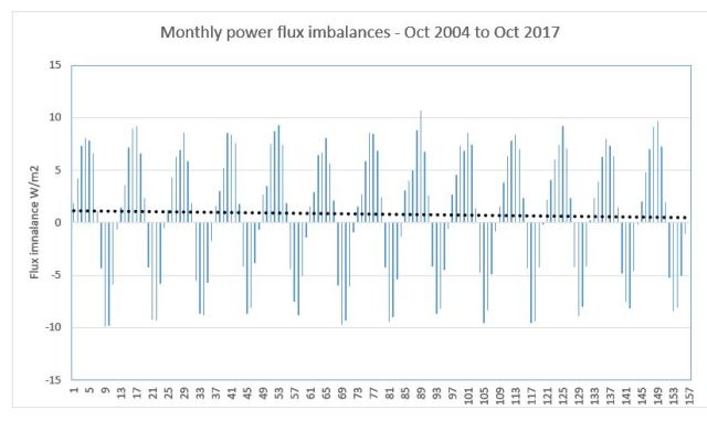
Figure 2: Monthly power flux imbalances – average monthly power flux in less power flux out
The eccentricity of the Earth’s orbit is currently 0.0167 – quite simply the difference between the actual orbit and a circular orbit at perihelion and aphelion. Cooler northern hemisphere summers and warmer winters – increasing NH summer snow survival and the risk of runaway ice sheet feedbacks and a new ice age.

Figure 3 Earth’s current orbital eccentricity
The result is a very large annual variation in energy from the Sun – the energy in component. Annual variability has significant implications for ocean heat change. Ocean heat does not change slowly as a result of greenhouse gases and thermal inertia but warms and cools rapidly in response to the very large annual signal.

Figure 4: Raw incoming solar power flux
There are very much smaller and longer term changes seen in ‘anomalies’. In which can be seen the approximately 11 year solar cycle as well as minor changes in solar intensity.

Figure 5: Incoming solar energy with the large annual signal removed
Net energy out – negative (SW+LW) – shows warming up by convention. The annual orbital cycle and longer term solar intensity change is modulated by changes from cloud, ice, vegetation, dust, greenhouse gases… Change it does – and in both IR and SW – in response to both the flow of energy through the system and dynamic internal responses.

Figure 6: Raw Net outgoing energy
There are many and complex responses that emerge spontaneously in the climate system – such as the cool 2008 Pacific anomalies. This system is the dominant source of cloud change (Clement et al 2009) and planetary hydrology. It shifts between warmer and cooler sea surface temperature states at a 20 to 30 year beat – a solar driven periodicity that seems likely connected to the approximately 22 year Hale Cycle of solar magnetic reversal.
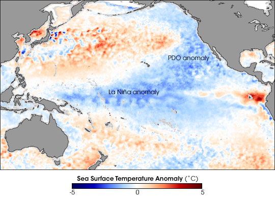
Figure 7: Pacific Ocean cool surface temperature anomalies – source NASA Earth Observatory
Outgoing energy is modulated by Rayleigh–Bénard convection in a fluid (the atmosphere) heated from below. Closed cloud cells – high albedo – tend to form over cold surfaces and open cell – low albedo – over warm (Koren et al 2017).
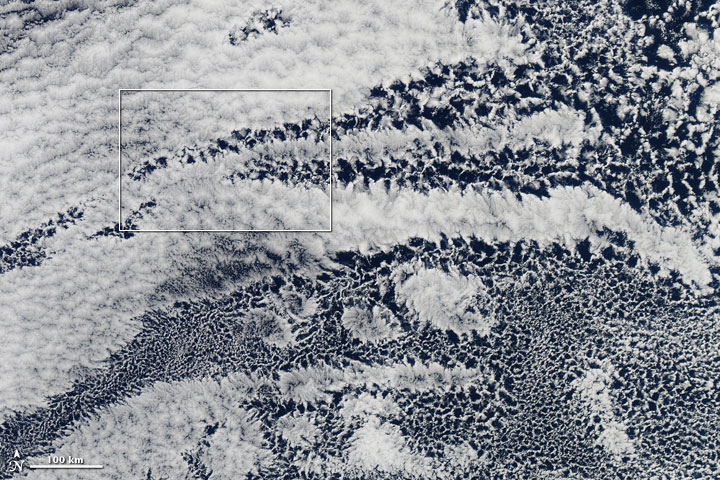

Figure 8: Closed and open cell cloud in satellite imagery over the Pacific Ocean – source NASA Earth Observatory
Decadal variability of clouds is an active area of research – e.g. Silvers et al 2017, Zhou et al 2018, Colman et al 2016, Colman and Power 2018 and XMoy et al (2002) present the record of sedimentation shown below which is strongly influenced by ENSO variability. It is based on the presence of greater and less red sediment in a lake core. More sedimentation is associated with a warm eastern Pacific surface. It has continuous high resolution coverage over 11,000 years. It shows periods of high and low El Niño intensity alternating with a period of about 2,000 years. There was a shift from La Niña dominance to El Niño dominance some 5000 years ago that was identified by Tsonis 2009 as a chaotic bifurcation – and is associated with the drying of the Sahel. There is a period around 3,500 years ago of high El Niño intensity associated with the demise of the Minoan civilisation (Tsonis et al, 2010). Red intensity was frequently in excess of 200 – for comparison red intensity in 1997/98 was 99.

Figure 9: Laguna Pallcacocha ENSO proxy – greater red intensity shows El Niño conditions (Source: Tsonis, 2009 – after Moy et al 2002)
Like flows in the Nile River – on which Pacific variability projects – the changes are not random noise in the climate system – that would sum to zero – but the product of dynamical complexity showing state regimes and globally coupled climate shifts at many scales. This inevitably leads to modulation of the global energy budget over many millennia at least.

Figure 10: Random vs dynamical climate change – after D. Koutsoyiannis
On the very short CERES record net energy out – the sum of SW and IR power fluxes over time – is the dominant term on the right hand side of the global energy equation. Net TOA power flux is warming up by convention – in what was a warming trend in net CERES data.
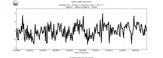
Figure 11: Net TOA power flux
Reflected SW responds to changes int incoming SW, cloud and north/south ocean/land asymmetry. In contrast to the net graph up is more energy reflected back to space – or in the IR data higher emissions – and a cooling planet.
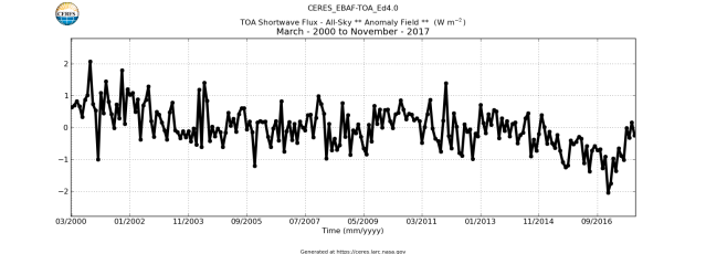
The cloud signal shows an anti-correlated relationship of IR and SW. Less cloud reflects less light but allows more IR to escape. With low marine strato-cumulus cloud SW dominates. There are land use, water vapor, aerosols, rain… and many other changes . But cloud impedes IR emissions and reflect SW. The IR anomalies at the bottom are a mirror of SW anomalies showing the role of cloud in 21st century changes in the energy budget.
(a)
(b)
 Figure 12: SW (a) and IR (b) TOA power flux
There is less reflected light in the early years followed by little net change and a recent warming associated with a warm eastern Pacific. The IR data on the other hand shows cooling in the early record, little change in the middle and more cooling at the end. The mirror image of SW and IR energy changes show that cloud was the dominant source of energy change in the climate system in the 21st century. Very little surface warming – and little of that not associated with EL Ninos – implies that the source of cloud change was not AGW cloud feedbacks. This is not to say that AGW is not buried somewhere in there amidst the large natural TOA power flux fluctuations resulting from ocean and atmospheric circulation changes (Loeb et al 2012). Nor that there isn’t a risk of adverse regimes initiated by greenhouse gases emerging from the dynamical complexity of the Earth system.

Very interesting, thank you
Reblogged this on Climate Collections.