The Unstable Math of Michael Ghil’s Climate Sensitivity

The US National Academy of Sciences (NAS) defined abrupt climate change as a new climate paradigm as long ago as 2002. A paradigm in the scientific sense is a theory that explains observations. A new science paradigm is one that better explains data – in this case climate data – than the old theory. The new theory says that climate change occurs as discrete jumps in the system. Climate is more like a kaleidoscope – shake it up and a new pattern emerges – than a control knob with a linear gain. This article reviews abrupt change in simple systems, in a 1-D climate model and in the climate system at multi-decadal timescales.

This idea is the most modern – and powerful – in climate science and has profound implications for the evolution of climate this century and beyond. A mechanical analogy might set the scene.

Figure 1: Simple mechanical analogy (Source: NAS Committee on Abrupt Climate Change, 2002)

Many simple systems exhibit abrupt change. The balance above consists of a curved track on a fulcrum. The arms are curved so that there are two stable states where a ball may rest. ‘A ball is placed on the track and is free to roll until it reaches its point of rest. This system has three equilibria denoted (a), (b) and (c) in the top row of the figure. The middle equilibrium (b) is unstable: if the ball is displaced ever so slightly to one side or another, the displacement will accelerate until the system is in a state far from its original position. In contrast, if the ball in state (a) or (c) is displaced, the balance will merely rock a bit back and forth, and the ball will roll slightly within its cup until friction restores it to its original equilibrium.’⁽¹⁾

In (a₁₎ the arms are displaced but not sufficiently to cause the ball to cross the balance to the other side. In (a₂) the balance is displaced with sufficient force to cause the ball to move to a new equilibrium state on the other arm. There is a third possibility in that the balance is hit with enough force to cause the ball to leave the track, roll off the table and under the sofa.

Ghil, 2013, explored the idea of abrupt climate change with an energy balance climate model that follows the evolution of global surface-air temperature with changes in the global energy balance. The plot below originates from work for Ghil’s Ph.D. thesis in 1975 and was reproduced in a 2013 World Scientific Review article to illustrate a dynamic definition of climate sensitivity in a climate system that exhibits abrupt change.

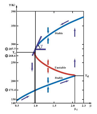
Figure 2: Solutions of an energy-balance model (EBM), showing the global-mean temperature (T) vs. the fractional change of insolation (μ) at the top of the atmosphere. (Source: Ghil, 2013)

The model has two stable states with two points of abrupt climate change – the latter at the transitions from the blue lines to the red from above and below. The two axes are normalized solar energy inputs μ (insolation) to the climate system and a global mean temperature. The current day energy input is μ = 1 with a global mean temperature of 287.7 degrees Kelvin. This is a relatively balmy 58.2 degrees Fahrenheit.

The 1-D climate model uses physically based equations to determine changes in the climate system as a result of changes in solar intensity, ice reflectance and greenhouse gases. With a small decrease in radiation from the Sun – or an increase in ice cover – the system becomes unstable with runaway ice feedbacks. Runaway ice feedbacks drive the transitions between glacial and interglacial states seen repeatedly over the past 2.58 million years. These are warm interludes – such as the present time – of relatively short duration and longer duration cold states. The transition between climate states is characterised by a series of step changes between the limits. It caused a bit of consternation in the 1970’s when it was realized that a very small decrease in solar intensity – or an increase in albedo – is sufficient to cause a rapid transition to an icy planet in this model ⁽²⁾.

Abrupt climate change is technically a chaotic bifurcation in a complex, dynamic system – equivalently a phase transition, a catastrophe (in the sense of René Thom), or a tipping point. These are all terms that are used in relation to the theory of deterministic chaos that originated with the work of Edward Lorenz in the 1960’s. Lorenz started his convection model calculation in the middle of a run by inputting values truncated to three decimal places in place of the original six. By all that was known – it should not have made much of a difference. The rest is history in the discovery of chaos theory as the third great idea – along with relativity and quantum mechanics – of 20^th century physics. It has applications in ecology, physiology, economics, electronics, weather, climate, planetary orbits and much else. In climate it is driving a new math of networked systems.

‘Technically, an abrupt climate change occurs when the climate system is forced to cross some threshold, triggering a transition to a new state at a rate determined by the climate system itself and faster than the cause. Chaotic processes in the climate system may allow the cause of such an abrupt climate change to be undetectably small…

Modern climate records include abrupt changes that are smaller and briefer than in paleoclimate records but show that abrupt climate change is not restricted to the distant past.^’ (NAS, 2002)

Ghil’s model shows that climate sensitivity (γ) is variable. It is the change in temperature (ΔT) divided by the change in the control variable (Δμ) – the tangent to the curve as shown above. Sensitivity increases moving down the upper curve to the left towards the bifurcation and becomes arbitrarily large at the instability. The problem in a chaotic climate then becomes not one of quantifying climate sensitivity in a smoothly evolving climate but of predicting the onset of abrupt climate shifts and their implications for climate and society. The problem of abrupt climate change on multi-decadal scales is of the most immediate significance.

Ding, Hui et al (2013) have made major progress in predicting abrupt climate shifts based on analysis of the 1976/1977 and 1998/2001 climate shifts. Mojib Latif – Head of the Research Division: Ocean Circulation and Climate Dynamics -Helmholtz Centre for Ocean Research Kiel has commented publicly on the research. ‘The winds change the ocean currents which in turn affect the climate. In our study, we were able to identify and realistically reproduce the key processes for the two abrupt climate shifts. We have taken a major step forward in terms of short-term climate forecasting, especially with regard to the development of global warming.’ However, ‘since the reliability of those predictions is still at about 50%, you might as well flip a coin.’ Numerical prediction of climate shifts using powerful climate models is now as accurate as tossing a coin – although perhaps we should not make light of such a difficult problem in climate science.

Abrupt climate change in the modern record explains observations that have been a puzzle for decades – notably the Pacific climate shift of 1976/1977. Tsonis et al (2007) used a mathematical network approach to analyze abrupt climate change on decadal timescales. Ocean and atmospheric indices – in this case the El Niño Southern Oscillation (ENSO), the Pacific Decadal Oscillation (PDO), the North Atlantic Oscillation (NAO) and the North Pacific Oscillation (NPO) – can be thought of as chaotic oscillators that are nodes on the network of the global climate system. The indices capture the major modes of climate variability. Tsonis and colleagues calculated the ‘distance’ between the indices. It was found that they would synchronize at certain times and then shift into a new state. It was noted that this was the first time that the mechanism – that is consistent with the theory of synchronized chaos in networks – was observed in a system the size of Earth’s climate. Swanson and Tsonis (2009) extended the research to the most recent climate shift at the turn of the millennium.

It is no coincidence that abrupt shifts in ocean and atmospheric circulation occur at the same time as changes in the trajectory of global surface temperature. Our ‘interest is to understand – first the natural variability of climate – and then take it from there. So we were very excited when we realized a lot of changes in the past century from warmer to cooler and then back to warmer were all natural,’ Tsonis said.

Four multi-decadal climate shifts were identified in the last century coinciding with changes in the surface temperature trajectory. Surface warming from 1909 to the mid 1940’s, cooling to 1976/77, warming to 1998 and cooling post the 1998/2001climate shift.

The multi-decadal climate shifts correspond precisely to changes in Pacific Ocean circulation, and in global hydrological patterns. The multi-decadal Pacific Ocean pattern can be seen in ENSO proxies for up to 1000 years (Vance et al, 2012). Abrupt changes between multi-decadal rainfall regimes were observed in river morphology in Australian rivers in the 1980’s (Erskine and Warner, 1988) and have been a cornerstone of Australian hydrology since – (e.g. Micevski et al, 2006, Power et al, 1999, Verdon et al, 2004).

In theory we then have a mechanism – albeit a complex one – that better explains abrupt shifts in paleoclimatic and modern records than a paradigm of slow responses to changes in forcing.

The abrupt shifts in Pacific Ocean circulation involve changes in the PDO in the north-eastern Pacific and coincident changes in the frequency and intensity of ENSO events. Increased frequency and intensity of La Niña occur with a cool mode PDO and vice versa (Verdon and Franks, 2006). The change in ocean circulation is associated with changes in wind, currents and cloud that change the energy dynamic of the planet. Cool decadal modes cool the planetary surface and warm modes add to the surface temperatures. A typical cool mode pattern is a cool ‘V’ across a significant part of the global tropics.

Figure 3: The cool ‘V’ characteristic of a cool Pacific Ocean decadal mode (Source: Current Operational SST Anomaly Charts – NOAA)

The PDO manifests as cool upwelling in the northeast Pacific – the upwelling brings with it cold bottom water and associated nutrients which results in decadal shifts in biological activity (e.g. Mantua, 1997). The northeast Pacific stayed cool from the 1940’s to 1976/1997, warm to 1998 and cool again since.

Figure 4: Pacific Decadal Oscillation (Source: Pacific Decadal Oscillation (PDO) | Teleconnections | National Climatic Data Center (NCDC))

ENSO has the same tempo with increased frequency and intensity of La Niña to 1978/1977, El Niño to 1998 and La Niña since. This is most easily seen in Claus Wolter’s multivariate ENSO index which incorporates sea-level pressure, surface wind, sea surface temperature, surface air temperature and total cloudiness fraction of the sky.

Figure 5: ENSO Index (Source: Earth System Research Laboratory)

Multi-decadal variability in the Pacific is defined as the Interdecadal Pacific Oscillation (e.g. Folland et al,2002, Meinke et al, 2005, Parker et al, 2007, Power et al, 1999) – a proliferation of oscillations it seems. The latest Pacific Ocean climate shift in 1998/2001 is linked to increased flow in the north (Di Lorenzo et al, 2008) and the south (Roemmich et al, 2007, Qiu, Bo et al 2006)Pacific Ocean gyres. Roemmich et al (2007) suggest that mid-latitude gyres in all of the oceans are influenced by decadal variability in the Southern and Northern Annular Modes (SAM and NAM respectively) as wind driven currents in baroclinic oceans (Sverdrup, 1947).

There is a growing literature on the potential for stratospheric influences on climate (e.g. Matthes et al 2006, Gray et al 2010, Lockwood et al 2010, Scaife et al 2012) due to warming of stratospheric ozone by solar UV emissions. Models incorporating stratospheric layers – despite differing greatly in their formulation of fundamental processes such as atmosphere-ocean coupling, clouds or gravity wave drag – show consistent responses in the troposphere. Top down modulation of SAM and NAM by solar UV has the potential to explain otherwise little understood variability at decadal to much longer scales in ENSO.

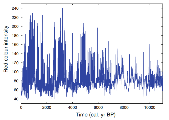
Figure 6: Laguna Pallcacocha, ENSO proxy – greater red intensity shows El Niño conditions (Source: Tsonis, 2009)

Moy et al (2002) present the record of sedimentation shown above which is strongly influenced by ENSO variability. It is based on the presence of greater and less red sediment in a lake core. More sedimentation is associated with El Niño. It has continuous high resolution coverage over 12,000 years. It shows periods of high and low ENSO activity alternating with a period of about 2,000 years. There was a shift from La Niña dominance to El Niño dominance that was identified by Tsonis 2009 as a chaotic bifurcation – and is associated with the drying of the Sahel. There is a period around 3,500 years ago of high ENSO activity associated with the demise of the Minoan civilisation (Tsonis et al, 2010). It shows ENSO variability considerably in excess of that seen in the modern period.

Swanson and Tsonis (2009) suggest that decadal surface cooling and warming results from a change in energy uptake in the deep oceans or a change in cloud and water vapour dynamics. Both seem likely. In the simplest case the cooler or warmer water surface loses less or more of the heat gained from sunlight and so the oceans warm and cool.

In the latter case – cloud cover seems increasingly likely to be a significant factor in the Earth’s energy dynamic. Loeb (2012) shows that large changes in the Earth’s energy balance at top of atmosphere occur with changes in ocean and atmospheric circulation. However, CERES commenced operation just after the 1998/2001 climate shift.

Earlier satellite data (International Satellite Cloud Climatology Project (ISCCP-FD) | NASA) shows a substantial step increase in cloud at the turn of the century. Pallé (2009) made photometric observations of light reflected from the Earth onto the moon from 1998. Short term changes in global reflectance is for the most part cloud changes. A climatologically significant step increase in albedo was observed at the turn of the century.

Although a significant factor in global climate on the scale of decades – the Pacific Ocean modes are part of a global climate system that is variable at many scales in time and space.

In the words of Michael Ghil (2013) the ‘global climate system is composed of a number of subsystems – atmosphere, biosphere, cryosphere, hydrosphere and lithosphere – each of which has distinct characteristic times, from days and weeks to centuries and millennia. Each subsystem, moreover, has its own internal variability, all other things being constant, over a fairly broad range of time scales. These ranges overlap between one subsystem and another. The interactions between the subsystems thus give rise to climate variability on all time scales.’

The theory suggests that the system is pushed by greenhouse gas changes and warming – as well as solar intensity and Earth orbital eccentricities – past a threshold at which stage the components start to interact chaotically in multiple and changing negative and positive feedbacks – as tremendous energies cascade through powerful subsystems. Some of these changes have a regularity within broad limits and the planet responds with a broad regularity in changes of ice, cloud, Atlantic thermohaline circulation and ocean and atmospheric circulation.

Dynamic climate sensitivity implies the potential for a small push to initiate a large shift. Climate in this theory of abrupt change is an emergent property of the shift in global energies as the system settles down into a new climate state. The traditional definition of climate sensitivity as a temperature response to changes in CO2 makes sense only in periods between climate shifts – as climate changes at shifts are internally generated. Climate evolution is discontinuous at the scale of decades and longer.

In the way of true science – it suggests at least decadal predictability. The current cool Pacific Ocean state seems more likely than not to persist for 20 to 30 years from 2002. The flip side is that – beyond a decade or so – the evolution of the global mean surface temperature may hold surprises on both the warm and cold ends of the spectrum (Swanson et al, 2009).

Current Operational SST Anomaly Charts – Office of Satellite and Product Operations – 2014. Available at: http://www.ospo.noaa.gov/Products/ocean/sst/anomaly/. [Accessed 13 June 2014].

Di Lorenzo, E., Schneider, N., Cobb, K. M., Chhak, K., Franks, P. J. S., Miller A. J., McWilliams, J. C., Bograd S. J., Arango H., Curchister E., Powell T. M. and P. Rivere, 2008: North Pacific Gyre Oscillation links ocean climate and ecosystem change. Geophys. Res. Lett., 35, L08607, doi:10.1029/2007GL032838.

Ding, Hui, Richard J. Greatbatch, Mojib Latif, Wonsun Park, Rüdiger Gerdes, 2013: Hindcast of the 1976/77 and 1998/99 climate shifts in the pacific. J. Climate, 26, 7650–7661. http://dx.doi.org/10.1175/JCLI-D-12-00626.1

Earth System Research Laboratory – PSD – 2014. Available at: http://www.esrl.noaa.gov/psd/enso/mei/. [Accessed 13 June 2014].

Enric Palle Home page. 2014. Available at: http://www.iac.es/galeria/epalle/. [Accessed 14 June 2014]

Erskine, W., Warner, R., 1988. Geomorphic effects of alternating flood-and drought-dominated regimes on the N.S.W. coastal rivers, in Warner, R. F. (Ed.), Fluvial Geomorphology in Australia, Academic Press, Sydney, 223–244, ISBN 0127356606, 9780127356600

Folland, C.K., J.A. Renwick, M.J. Salinger and A.B. Mullan, 2002: Relative influences of the Interdecadal Pacific Oscillation and ENSO on the South Pacific Convergence Zone. Geophys. Res. Lett., 29 (13): 10.1029/2001GL014201. Pages 21-1 – 21-4, DOI: 10.1029/2001GL014201

Gray, L. J., Beer, J., Geller, M., Haigh, J. D., Lockwood, M., Matthes, K., Cubasch, U., Fleitman, D., Harrison, G., Luterbacher, J. Meehl, G. A.: Solar influences on climate, 2010, Reviews of Geophysics, Volume 48, Issue 4, DOI: 10.1029/2009RG000282

International Satellite Cloud Climatology Project (ISCCP-FD) – NASA – 2014. Available at: http://isccp.giss.nasa.gov/projects/browse_fc.html. [Accessed 13 June 2014].

Lockwood, M., Bell, C., Woollings, T., Harrison, R. G., Gray, L. J. and Haigh, J. D.: Top-down solar modulation of climate: evidence for centennial-scale change, Environ. Res. Lett. 5 (July-September 2010) 034008 doi:10.1088/1748-9326/5/3/034008
Loeb, N. G., Kato, S., Wenying, S., Wong, T., Rose, F. G., Doeling, D. R., Norris, J. R., Xianglei, H., 2012: Advances in Understanding Top-of-Atmosphere Radiation Variability from Satellite Observations, Surveys in Geophysics , Volume 33, Issue 3-4, pp 359-385, ISSN: 0169-3298 (Print) 1573-0956 (Online)

Mantua, N.J., Hare, S.R., Zhang, Y., Wallace, J.M. and R.C. Francis, 1997: A Pacific interdecadal climate oscillation with impacts on salmon production. Bull. Amer. Met Soc., 78, 1069-1079

Matthes, K., Kurada, Y., Kunihiko, K. and Langematz, U., 2006: Transfer of the solar signal from the stratosphere to the troposphere: Northern winter Journal of Geophysical Research: Atmospheres (1984–2012), DOI: 10.1029/2005JD006283

Micevski, T., Franks, S. W., Kuczera, G., 2006, Multidecadal variability in coastal eastern Australian flood data, Journal of Hydrology, Volume 327, Issues 1–2, 30 July 2006, Pages 219-225, DOI: 10.1016/j.jhydrol.2005.11.017

Moy, C. M., Seltzer, G. O., Rodbell D. T. and Anderson, D. M., 2002, Variability of El Niño/Southern Oscillation activity at millennial timescales during the Holocene epoch Nature 420, 162-165 (14 November 2002) | doi:10.1038/nature01194

Meinke, H., deVoil, P., Hammer, G.L., Power, S., Allan, R., Stone, R.C., Folland, C. and Potgieter, A., 2005: Rainfall variability at decadal and longer time scales: signal or noise? J. Climate, 18, 89-96.

Pallé, E., 2019: Inter‐annual trends in earth’s reflectance 1999–2007, AIP Conf. Proc. 1100, 486 (2009); http://dx.doi.org/10.1063/1.3117027

Power, S., T. Casey, C. Folland, A. Colman and V. Mehta, 1999, Inter-decadal modulation of the impact of ENSO on Australia, Climate Dynamics 15, 319-324, ISSN: 0930-7575

Roemmich, D., J. Gilson, R. Davis, P. Sutton, S. Wijffels, S. Riser, 2007: Decadal Spinup of the South Pacific Subtropical Gyre. J. Phys. Oceanogr., 37, 162–173. doi: http://dx.doi.org/10.1175/JPO3004.1

Pacific Decadal Oscillation (PDO) – Teleconnections – National Climatic Data Center (NCDC) – 2014. Available at: http://www.ncdc.noaa.gov/teleconnections/pdo.php. [Accessed 13 June 2014].

Parker, D.E., Folland C.K., A.A. Scaife, A. Colman, J. Knight, D. Fereday, P. Baines and D. Smith, 2007: Decadal to interdecadal climate variability and predictability and the background of climate change. JGR (Atmos), 112,.D18115 doi 10.1029/2007JD008411.

Power, S., Casey, T., Folland, C.K., Colman, A and V. Mehta, 1999: Inter-decadal modulation of the impact of ENSO on Australia. Climate Dynamics, 15, 319-323.

Qiu, Bo, Shuiming Chen, 2006: Decadal variability in the large-scale sea surface height field of the south pacific ocean: observations and causes. J. Phys. Oceanogr., 36, 1751–1762. doi: http://dx.doi.org/10.1175/JPO2943.1<

Scaife, A. A., Spangehi, T., Cubasch, U., Langematz, U., Akiyoshi, H., Bekki, S Butchart, N., Chipperfield, M. P., Gettelman, A., Hardiman, S. C., Michou, M., Rozanov, E. and Shepherd, T. G., 2012: Climate change projections and stratosphere–troposphere interaction. Climate Dynamics, 38 (9-10). pp. 2089-2097. ISSN 0930-7575

Swanson, K. L., and Tsonis, A. A.,2009, Has the climate recently shifted?Geophys. Res. Lett., 36, DOI: 10.1029/2008GL037022

Sverdrup, H. U., 1947, Wind-driven currents in a baroclinic ocean; with appliations to the equatorial currents of the eastern Pacific, PNAS, vol. 33 no. 11

Tsonis, A. A., Swanson, K. L., Sugihara, G. and Tsonis, P. A, 2010: Climate change and the demise of Minoan civilization, 2010, Clim. Past, 6, 525-530, 2010, doi:10.5194/cp-6-525-2010 US National Academy of Sciences, Committee on Abrupt Climate Change, 2002, Abrupt Climate Change: inevitable surprises, NAP: ISBN 0-309-07434-7

Tsonis. A. A., 2009: Dynamical changes in the ENSO system in the last 11,000 years, Climate Dynamics, Volume 33, Issue 7-8, pp 1069-1074: 10.1007/s00382-008-0469-4

Tsonis, A. A. Swanson, K., Kravtsov, S., 2007: A new dynamical mechanism for major climate shifts, Geophysical Research Letters, Geophys. Res. Lett. 34, DOI: 10.1029/2007GL030288

Vance, T. .R, van Ommen, T.D., Curran, M. A. J., Plummer, C. T. and Moy, AD, 2012, A Millennial Proxy Record of ENSO and Eastern Australian Rainfall from the Law Dome Ice Core, East Antarctica, Journal of Climate, 26, (3) pp. 710–725, http://dx.doi.org/10.1175/JCLI-D-12-00003.1

Verdon, D. C., Franks, S. W., 2006, Long-term behaviour of ENSO: Interactions with the PDO over the past 400 years inferred from paleoclimate records, Geophysical Research Letters, Volume 33, Issue 6, March 2006, DOI: 10.1029/2005GL025052

Verdon, D. C. and Wyatt, A. M. and Kiem, A..S. and Franks, S. W., Multidecadal variability of rainfall and streamflow: Eastern Australia, Water Resources Research, 40 Article W10201. ISSN 1944-7973 (2004)