The illusion of climate cycles

“Using past variations of solar activity measured by cosmogenic isotope abundance changes, analogue forecasts for possible future solar output have been calculated. An 8% chance of a return to Maunder Minimum-like conditions within the next 40 years was estimated in 2010 (ref. 2). The decline in solar activity has continued, to the time of writing, and is faster than any other such decline in the 9,300 years covered by the cosmogenic isotope data¹.” Sarah Ineson et al, 2014, Regional climate impacts of a possible future grand solar minimum

The chances of Maunder Minimum-like conditions emerging is now put at 20%.  Varying solar output has been hypothesized to be due to the eccentric path of the solar system barycenter driving the solar magneto.  But it is also emerges from turbulent  fluid dynamics within the Sun.  Poincaré’s 3 body problem and Lorenz’s butterfly reveal dynamical complexity at the heart of both.

Cosmic ray intensity is inversely related to solar intensity – in which UV radiation is a prominent variable.  Some 19% of the total change in the 1980’s solar max to min.   What we can see in the cosmogenic isotope record is variability at all scales – with an interesting transition to higher solar intensity a little over 5,000 years ago – that has been linked to the mid-Holocene ENSO transition.  The last thousand years has seen a centennial decline in solar activity and a 20th century peak.  The strictly aperiodic solar activity variability driven by chaotic orbits and turbulence are insufficient to cause the climate changes that have been seen.  What it may do is trigger non-linear planetary responses.

“Since irradiance variations are apparently minimal, changes in the Earth’s climate that seem to be associated with changes in the level of solar activity—the Maunder Minimum and the Little Ice age for example—would then seem to be due to terrestrial responses to more subtle changes in the Sun’s spectrum of radiative output. This leads naturally to a linkage with terrestrial reflectance, the second component of the net sunlight, as the carrier of the terrestrial amplification of the Sun’s varying output.”  Shortwave forcing of the Earth’s climate: modern and historical variations in the Sun’s irradiance and the Earth’s reflectance, P.R. Goode, E. Palle, J. Atm. and Sol.-Terr. Phys., 69,1556, 2007. 

Over the long term ice sheets are the major part of solar amplification – and over the short term we are looking at cloud cover changes in response to changes in ocean and atmosphere circulation.  “Closed cells tend to be associated with the eastern part of the subtropical oceans, forming over cold water (upwelling areas) and within a low, stable atmospheric marine boundary layer (MBL), while open cells tend to form over warmer water with a deeper MBL.”  Ilan Koren et al, 2017, Exploring the nonlinear cloud and rain equation  The region of the planet where sea surface temperature change most dramatically is over a large part of the Pacific Ocean.  Rayleigh-Benard Convection cloud physics result in changes in planetary albedo.

What can be seen over 9,400 years is variability rather than an illusion of regularity.    As would indeed be anticipated from the fundamental physics of complexity.   “From the smallest scales to the largest, there exists an apparent conundrum: nature is both simple and complex.  From apparent disorder, order emerges. This elegance in nature lies at the heart of my research interests.”  Marcia Wyatt

The authors of the paper I started with suggest that solar UV/ozone chemistry affects are translated through atmospheric pathways to modulate surface pressure at the poles.  Southern and northern annular modes are thus partially under the thrall of solar variability.  There are other factors influencing polar surface pressure.  When pressures are high in low solar intensity winds and storms are pushed into lower latitudes.  Winds and storms spin up sub-polar gyres in the world’s oceans with dramatic effects on deep ocean upwelling in the eastern Pacific.  None of this can be analysed in terms of simple correlation.  It cannot be modeled because the numerical functions do not exist.  It can be approached as network math with atmospheric and oceanic indices as nodes of chaotic oscillators on a global spanning  spatio-temporal network.  Or perhaps as a signal propagating around the planet using the Multichannel Singular Spectrum Analysis of Marcia Wyatt and Judith Curry.

At a millennial scale the state of the Pacific Ocean superficially resembles the 1000 year cosmogenic isotope record – but the response is dynamic and nonlinear.

Tessa Vance et al, 20213, A Millennial Proxy Record of ENSO and Eastern Australian Rainfall from the Law Dome Ice Core, East Antarctica

“Over the last 1010 yr, the LD summer sea salt (LD_SSS) record has exhibited two below-average (El Niño–like) epochs, 1000–1260 ad and 1920–2009 ad, and a longer above-average (La Niña–like) epoch from 1260 to 1860 ad. Spectral analysis shows the below-average epochs are associated with enhanced ENSO-like variability around 2–5 yr, while the above-average epoch is associated more with variability around 6–7 yr. The LD_SSS record is also sig nificantly correlated with annual rainfall in eastern mainland Australia. While the correlation displays decadal-scale variability similar to changes in the interdecadal Pacific oscillation (IPO), the LD_SSS record suggests rainfall in the modern instrumental era (1910–2009 ad) is below the long-term average.” op. cit.

The change in the beat of ENSO variability around the turn of the 20th century suggests perhaps a slight step change in the solar UV control variable at that time.   The persistence of the 20 to 30 year signal may be related to the quasi 22 year cycle of heliomagnetic reversals – with weaker 11 year cycles following stronger and with dynamic leads and lags.  An intriguing possibility – with declining solar intensity – is a return to a  La Niña-like epoch seen before the mid-Holocene transition.

Moy et al (2002) present the record of sedimentation in a South American lake shown below (panel b) – which is strongly influenced by Pacific Ocean variability. It is based on the presence of greater and less red sediment in a lake core. More sedimentation is associated with higher rainfall in El Niño conditions. It has continuous high resolution coverage over 11,500 years. It shows periods of high and low El Niña activity alternating with a period of about 2,000 years.  And there is the shift from La Niña dominance to El Niño dominance a little over 5,000 years ago that was identified by Tsonis 2009 as a chaotic bifurcation – and is associated with the drying of the Sahel. There is a period around 3,500 years ago of high El Niño intensity – red intensity greater than 200 –   associated with the demise of the Minoan civilisation (Tsonis et al, 2010).  For comparison – red intensity in the 98/99 El Niño was 99.

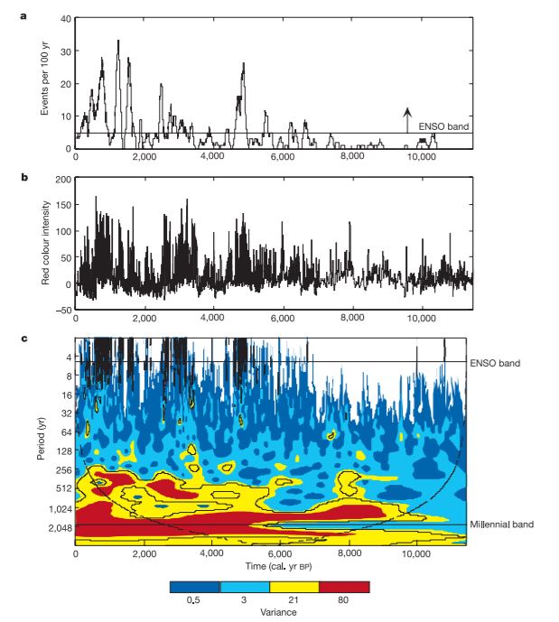
The time “series and wavelet power spectrum documenting changes in ENSO
variability during the Holocene. a, Event time series created using the event model (see
Methods), illustrating the number of events in 100-yr overlapping windows. The solid line denotes the minimum number of events in a 100-yr window needed to produce ENSO and variance.  b, Most recent 11,500 yr of the time series of red colour intensity. The absolute red colour intensity and the width of the individual laminae do not correspond to the intensity of the ENSO event. c, Wavelet power spectrum calculated using the Morlet wavelet on the time series of red colour intensity (b). Variance in the wavelet power spectrum (colour scale) is plotted as a function of both time and period. Yellow and red regions indicate higher degrees of variance, and the black line surrounds regions of variance that exceed the 99.98% confidence level for a red noise process (at 4–8-yr period, the regions of significant variance are shown black rather than outlined). Variance below the dashed line has been reduced owing to the wavelet approaching the end of the finite time series. Horizontal lines indicate average timescale for the ENSO and millennial bands.”  Christopher Moy et al, 2002, Variability of El Niño/Southern Oscillation activity at millennial timescales during the Holocene epoch

If as suspected solar activity evolves in response to an incalculable solar system N-body orbital problem – and this is further modulated through internal fluid dynamics of the Sun – cyclic behavior as such is impossible.   How far it departs from the cyclical expectations of classical mechanics is unknowable – but depart it does.  Solar variability as well triggers nonlinear responses in the planetary system.   In geophysical data the reality is  Hurst-Kolmogorov  effects – regimes and abrupt shifts.   Wavelet analysis – as above – will give you broad spectral peaks – but this is just math and not proof of anything.  Geophysics is required to understand the climate system and how it may change in future.  Nor do cycles say anything about how greenhouse gases may perturb flow and change turbulent patterns in Earth’s spatio-temporal chaotic flow field.  It may change them a little or a lot – it depends.